Double-Difference Earthquake Relocation
Introduction
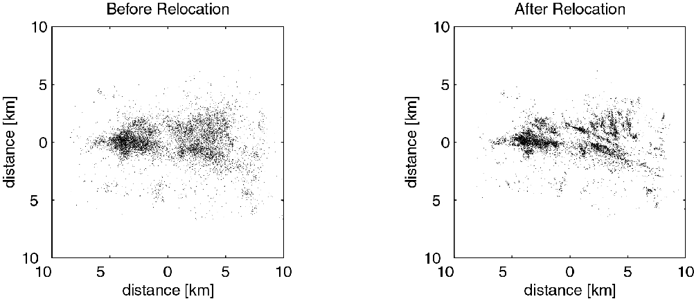
Double-difference earthquake relocation algorithm was developed to improve the location accuracy in the presence of measurement uncertainties when we locate earthquakes in the previous tutorial. It is based on the iterative least-square method, using the time difference between observed and predicted phase arrivals for event pairs recorded by a common station, some uncertainties can be canceled to derive high-accuracy hypocenter locations over large distance. Figure below shows a comparison of ~10,000 earthquake locations (left panel) and double-difference locations (right panel) during the 1997 seismic crisis in the Long Valley caldera (Waldhauser, 2001).
In this tutorial, we’ll go through the powerful earthquake double-difference location method. To better convey the key conception of the method, we simplify the model to avoid it runs too complicated to be understood. We’ll use:
one-layer homogeneous velocity model to get rid of complicated ray-tracing.
2-D X-Z plane rather than 3-D X-Y-Z to decrease complexity
P arrivals only
After this tutorial, besides the understanding of key concepts in Double-Difference location, you will also find that model expands from 2-D to 3-D, from one-layer to multi-layers, from P to P&S arrivals, the key processing remains the same.
Note
Contents of this tutorial
Initiation process
Double difference method
Iterative double-difference method
Authors: ZI Jinping, SONG Zilin, Earth Science Sytem Program, CUHK.
Testers, XIA Zhuoxuan, Sun Zhangyu, Earth Science Sytem Program, CUHK.
Initiation
Preparation for Environment
import numpy as np
import time
import matplotlib.pyplot as plt
from matplotlib.patches import Polygon
from scipy.sparse.linalg import lsqr
from scipy.sparse import csc_matrix
Note
def iter_loc(hyc_loop,stas,d,V,niter=10):
    """
    Iterative aboslute earthquake location using least-square method,
    refer to absolute earthquake location python tutorial.
    Parameters:
    | hyc_loop: hypocenter for iteration
    |     stas: array containing station information
    |        d: the observed arrival time
    |        V: the velocity
    |    niter: maximum number of iteration
    """
    k = 0
    while k <= niter:
        dcal = np.zeros((d.shape[0],1))
        for i in range(d.shape[0]):
            dx = stas[i,0]-hyc_loop[0]
            dz = stas[i,1]-hyc_loop[1]
            dcal[i,0] = np.sqrt(dx**2+dz**2)/V+hyc_loop[2]
        delta_d = d - dcal
        e2 = 0
        for i in range(delta_d.shape[0]):
            e2 += delta_d[i,0]**2
        print(f"Iteration {format(k,'2d')} square error: ",format(e2,'13.8f'))

        # >>>>> Build G matrix >>>>>>
        G = np.zeros((d.shape[0],3))
        G[:,2]=1
        for i in range(d.shape[0]):
            for j in range(2):
                denomiter = np.sqrt((hyc_loop[0]-stas[i,0])**2+(hyc_loop[1]-stas[i,1])**2)
                G[i,j]=(hyc_loop[j]-stas[i,j])/denomiter/V

        # >>>>> Invert the m value >>>>
        GTG = np.matmul(G.T,G)
        GTG_inv = np.linalg.inv(GTG)
        GTG_inv_GT = np.matmul(GTG_inv,G.T)
        delta_m = np.matmul(GTG_inv_GT,delta_d)

        # >>>>> Update the hypocenter loop >>>>>
        hyc_loop = np.add(hyc_loop,delta_m.ravel())
        k = k+1

        # >>>>> End the loop if error is small >>>>>
        if e2<0.00000001:
            break

    sigma_d = np.std(delta_d)
    var = sigma_d**2*(d.shape[0])/(d.shape[0]-4)
    sigma_m2 = var * GTG_inv
    return hyc_loop, sigma_m2

def present_loc_results(hyc,sig_square=None,std_fmt='.2f'):
    """
    Print earthquake location results, refer to absolute earthquake location
    for reference
    Parameters:
    |         hyc: hypocenter
    |sig_square: squared convariance
    """
    _x = format(np.round(hyc[0],4),format("6.2f"))
    _z = format(np.round(hyc[1],4),format("6.2f"))
    _t = format(np.round(hyc[2],4),format("6.2f"))
    if not isinstance(sig_square,np.ndarray):
        print("x = ",_x," km")
        print("z = ",_z," km")
        print("t = ",_t," s")
    else:
        stdx = sig_square[0,0]**0.5
        _stdx = format(np.round(stdx,4),std_fmt)
        stdz = sig_square[1,1]**0.5
        _stdz = format(np.round(stdz,4),std_fmt)
        stdt = sig_square[2,2]**0.5
        _stdt = format(np.round(stdt,4),std_fmt)
        print("x = ",_x,"±",_stdx," km")
        print("z = ",_z,"±",_stdz," km")
        print("t = ",_t,"±",_stdt," s")

def matrix_show(*args,**kwargs):
    """
    Show matrix values in grids shape
    Parameters:cmap="cool",gridsize=0.6,fmt='.2f',label_data=True
    """
    ws = []
    H = 0
    str_count = 0
    ndarr_count = 0
    new_args = []
    for arg in args:
        if isinstance(arg,str):
            new_args.append(arg)
            continue
        if isinstance(arg,list):
            arg = np.array(arg)
        if len(arg.shape)>2:
            raise Exception("Only accept 2D array")
        if len(arg.shape) == 1:
            n = arg.shape[0]
            tmp = np.zeros((n,1))
            tmp[:,0] = arg.ravel()
            arg = tmp
        h,w = arg.shape
        if h>H:
            H=h
        ws.append(w)
        new_args.append(arg)
        ndarr_count += 1
    W = np.sum(ws)+len(ws)    # text+matrix+text+...+matrix+text
    if W<0:
        raise Exception("No matrix provided!")

    fmt = '.2f'
    grid_size = 0.6
    cmap = 'cool'
    label_data = True
    for arg in kwargs:
        if arg == "fmt":
            fmt = kwargs[arg]
        if arg == 'grid_size':
            grid_size = kwargs[arg]
        if arg == 'cmap':
            cmap = kwargs[arg]
        if arg == 'label_data':
            label_data = kwargs[arg]
    fig = plt.figure(figsize=(W*grid_size,H*grid_size))
    gs = fig.add_gridspec(nrows=H,ncols=W)

    wloop = 0
    matrix_id = 0
    for arg in new_args:
        if isinstance(arg,str):
            ax = fig.add_subplot(gs[0:H,wloop-1:wloop])
            ax.axis("off")
            ax.set_xlim(0,1)
            ax.set_ylim(0,H)
            ax.text(0.5,H/2,arg,horizontalalignment='center',verticalalignment='center')
        if isinstance(arg,np.ndarray):
            h,w = arg.shape
            hlow = int(np.round((H-h+0.01)/2))        # Find the height grid range
            hhigh = hlow+h
            wlow = wloop
            whigh = wlow+w
#            print("H: ",H,hlow,hhigh,"; W ",W,wlow,whigh)
            ax = fig.add_subplot(gs[hlow:hhigh,wlow:whigh])

            plt.pcolormesh(arg,cmap=cmap)
            for i in range(1,w):
                plt.axvline(i,color='k',linewidth=0.5)
            for j in range(1,h):
                plt.axhline(j,color='k',linewidth=0.5)
            if label_data:
                for i in range(h):
                    for j in range(w):
                        plt.text(j+0.5,i+0.5,format(arg[i,j],fmt),
                                 horizontalalignment='center',
                                 verticalalignment='center')
            plt.xlim(0,w)
            plt.ylim([h,0])
            plt.xticks([])
            plt.yticks([])
            wloop+=w+1
            matrix_id+=1
    plt.show()
Basic parameters
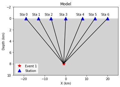
Set up station array, earthquake true location, wave-velocity and generate synthetic arrival time.
stas =np.array([[-20,0],[-14,0],[-8,0],[0,0],[8,0],[14,0],[20,0]]) # Station
stas =np.array([[-19,0],[-13,0],[-7,0],[0,0],[8,0],[14,0],[20,0]]) # Station
hyc1_true = np.array([-1,8,0])
Vtrue = 5
nsta = stas.shape[0]
dobs1 = np.zeros((nsta,1))
for i in range(dobs1.shape[0]):
    dx = stas[i,0]-hyc1_true[0]
    dz = stas[i,1]-hyc1_true[1]
    dobs1[i,0] = np.sqrt(dx**2+dz**2)/Vtrue+hyc1_true[2]
# Plot event, stations, and rays
fig,ax= plt.subplots(1,1)
plt.plot(hyc1_true[0],hyc1_true[1],'r*',ms=10,label='Event 1')
plt.plot(stas[:,0],stas[:,1],'b^',ms=10,label="Station")
for sta in stas:
    plt.plot([hyc1_true[0],sta[0]],[hyc1_true[1],sta[1]],'k-')

# Add grey background
nodes = [[-25,10],[25,10],[25,0],[-25,0]]
p = Polygon(nodes,facecolor='lightgrey')
for i in range(stas.shape[0]):
    sta = stas[i]
    plt.text(sta[0]-3,sta[1]-0.5,'Sta '+str(i))
plt.gca().add_patch(p)

# Set up plot elements
plt.xlim([-25,25])
plt.ylim([10,-2])
plt.xlabel("X (km)")
plt.ylabel("Depth (km)")
plt.title("Model")
plt.legend();
Absolute earthquake location
Initial location
The station which records the earliest waveform is closest to the hypocenter, so it is reasonable to start iteration:
The same x and y with the closest station;
Initial depth at 5 km;
Initial origin time 1 sec before the earliest arrival;
idx = np.argmin(dobs1)       # The index of station
dmin = np.min(dobs1)         # The minimum arrival time

hyc1_init = np.zeros(3);      # Init array
hyc1_init[0] = stas[idx,0];   # Set the same x,y with station
hyc1_init[1] = 5;                 # Set initial depth 5 km
hyc1_init[2] = dmin-1;        # Set initial event time 1s earlier than arrival
print("Initial trial parameters ","x: ",hyc1_init[0],"km; ","z: ",hyc1_init[1],"km; ","t: ", format(hyc1_init[2],'.4f')+" s")
hyc1_loop = hyc1_init.copy()
Initial trial parameters x: 0.0 km; z: 5.0 km; t: 0.6125 s
We can also define a function to get the initial location
def get_init_loc(dobs,stas,depth=5,gap_time=1):
    """
    Get initial earthquake location
    """
    dmin = np.min(dobs)         # The minimum arrival time
    idx = np.argmin(dobs)       # The index of observation

    hyc_init = np.zeros(3);      # Init array
    hyc_init[0] = stas[idx,0];   # Set the same x,y with station
    hyc_init[1] = depth;             # Set initial depth 5 km
    hyc_init[2] = dmin-gap_time;        # Set initial event time 1s earlier than arrival
    print("Initial trial parameters ","x: ",hyc_init[0],"km; ","z: ",hyc_init[1],"km; ","t: ", format(hyc_init[2],'.4f')+" s")
    return hyc_init
hyc1_init = get_init_loc(dobs1,stas)
Initial trial parameters x: 0.0 km; z: 5.0 km; t: 0.6125 s
Note
hyc1_abs, sigma_m2 = iter_loc(hyc1_loop,stas,dobs1,Vtrue)
present_loc_results(hyc1_abs,sigma_m2,std_fmt='.4f')
Iteration  0 square error:     0.83833287
Iteration  1 square error:     0.01411773
Iteration  2 square error:     0.00000020
Iteration  3 square error:     0.00000000
x =   -1.00 ± 0.0000  km
z =    8.00 ± 0.0000  km
t =    0.00 ± 0.0000  s
Velocity Error
In the calculation above, we use the true velocity (Vtrue) to conduct the inversion. However, in reality, the velocity we measure is more or less different from the true velocity, thus leading to some bias.
Note
Vp = 4.8
hyc1_abs, sigma_m2 = iter_loc(hyc1_init,stas,dobs1,Vp)
present_loc_results(hyc1_abs,sigma_m2,std_fmt='.4f')
print("True location (hyc1_true) ","x: ",hyc1_true[0],"km; ","z: ",hyc1_true[1],"km; ","t: ", format(hyc1_true[2],'.4f')+" s")
Note
Iteration  0 square error:     1.44386729
Iteration  1 square error:     0.03284725
Iteration  2 square error:     0.00078154
Iteration  3 square error:     0.00077835
Iteration  4 square error:     0.00077835
Iteration  5 square error:     0.00077835
Iteration  6 square error:     0.00077835
Iteration  7 square error:     0.00077835
Iteration  8 square error:     0.00077835
Iteration  9 square error:     0.00077835
Iteration 10 square error:     0.00077835
x =   -0.98 ± 0.0398  km
z =    8.90 ± 0.1464  km
t =   -0.24 ± 0.0204  s
True location (hyc1_true)  x:  -1 km;  z:  8 km;  t:  0.0000 s
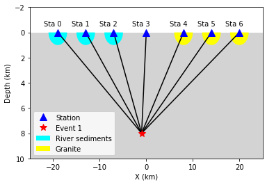
Station Delay
In near surface, the material velocity where stations are located might vary and lead to influence on the travel time, we call it Station delay. The River sediments are generally composed by not fully consolidated materials, their velocities are therefore low. A lower velocity will lead to a longer travel time, thus the actual arrival time will be later than estimated, here we call it Positive delay.
The Granite is igneous rock, its density is high with fast velocity. A higher velocity will lead to a shorter travel time, thus the actual arrival time will be earlier than estimated, we call it Negative delay.
In this tutorial, we set value of 0.05s for positive delay and -0.05s for negative delay.
semix = np.linspace(-1,1,101)
semiy = np.sqrt(1-semix**2)
semixy = np.zeros((101,2))
semixy[:,0] = semix
semixy[:,1] = semiy*0.5
for sta in stas:
    plt.plot([hyc1_true[0],sta[0]],[hyc1_true[1],sta[1]],'k')
station, = plt.plot(stas[:,0],stas[:,1],'b^',ms=10,label="Station")
event, = plt.plot(hyc1_true[0],hyc1_true[1],'r*',ms=10,label='Event 1')
nodes = [[-25,10],[25,10],[25,0],[-25,0]]
p = Polygon(nodes,facecolor='lightgrey')
plt.gca().add_patch(p)
for sta in stas[:3]:
    p_pos = Polygon(sta+semixy*2,facecolor='cyan')
    plt.gca().add_patch(p_pos)
for sta in stas[4:]:
    p_neg = Polygon(sta+semixy*2,facecolor='yellow')
    plt.gca().add_patch(p_neg)
for i in range(stas.shape[0]):
    sta = stas[i]
    plt.text(sta[0]-3,sta[1]-0.5,'Sta '+str(i))

plt.xlabel("X (km)")
plt.ylabel("Depth (km)")
plt.xlim([-25,25])
plt.ylim([10,-2])
plt.legend([station,event,p_pos,p_neg],["Station","Event 1","River sediments","Granite"]);
stas_delay = np.zeros((nsta,1))
stas_delay[:,0]= [0.05,0.05,0.05,0,-0.05,-0.05,-0.05]
Conduct inversion with delayed data
dobs1_delay = dobs1 + stas_delay
hyc1_abs_delay, sigma_m2 = iter_loc(hyc1_init,stas,dobs1_delay,Vp)
present_loc_results(hyc1_abs_delay,sigma_m2)
print("True location (hyc1_true) ","x: ",hyc1_true[0],"km; ","z: ",hyc1_true[1],"km; ","t: ", format(hyc1_true[2],'.4f')+" s")
Iteration  0 square error:     1.36803100
Iteration  1 square error:     0.03083627
Iteration  2 square error:     0.00074298
Iteration  3 square error:     0.00073813
Iteration  4 square error:     0.00073813
Iteration  5 square error:     0.00073813
Iteration  6 square error:     0.00073813
Iteration  7 square error:     0.00073813
Iteration  8 square error:     0.00073813
Iteration  9 square error:     0.00073813
Iteration 10 square error:     0.00073813
x =   -0.69 ± 0.04  km
z =    8.96 ± 0.14  km
t =   -0.24 ± 0.02  s
True location (hyc1_true)  x:  -1 km;  z:  8 km;  t:  0.0000 s
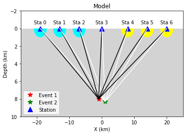
The second event
Now we consider a second event occurred close to the first event
hyc2_true = [1,8.3,1]
# Plot event, stations, and rays
fig,ax= plt.subplots(1,1)

# Add grey background
nodes = [[-25,10],[25,10],[25,0],[-25,0]]
p = Polygon(nodes,facecolor='lightgrey')
plt.gca().add_patch(p)

# Plot events
plt.plot(hyc1_true[0],hyc1_true[1],'r*',ms=10,label='Event 1')
plt.plot(hyc2_true[0],hyc2_true[1],'g*',ms=10, label="Event 2")


# Plot stations and rays
plt.plot(stas[:,0],stas[:,1],'b^',ms=10,label="Station")
for i in range(stas.shape[0]):
    sta = stas[i]
    plt.text(sta[0]-2,sta[1]-0.5,'Sta '+str(i))
    plt.plot([hyc1_true[0],sta[0]],[hyc1_true[1],sta[1]],'k-')
    plt.plot([hyc2_true[0],sta[0]],[hyc2_true[1],sta[1]],'w-')
    if i<3:
        p_pos = Polygon(sta+semixy*2,facecolor='cyan')
        plt.gca().add_patch(p_pos)
    if i>3:
        p_neg = Polygon(sta+semixy*2,facecolor='yellow')
        plt.gca().add_patch(p_neg)

# Set up plot elements
plt.xlim([-25,25])
plt.ylim([10,-2])
plt.xlabel("X (km)")
plt.ylabel("Depth (km)")
plt.title("Model")
plt.legend();
dobs2 = np.zeros((nsta,1))
for i in range(dobs2.shape[0]):
    dx = stas[i,0]-hyc2_true[0]
    dz = stas[i,1]-hyc2_true[1]
    dobs2[i,0] = np.sqrt(dx**2+dz**2)/Vtrue+hyc2_true[2]
hyc2_init = get_init_loc(dobs2,stas)
Initial trial parameters x: 0.0 km; z: 5.0 km; t: 1.6720 s
dobs2_delay = dobs2 + stas_delay
hyc2_abs, sigma_m2 = iter_loc(hyc2_init,stas,dobs2_delay,Vtrue)
present_loc_results(hyc2_abs,sigma_m2)
print("True location (hyc2_true) ","x: ",hyc2_true[0],"km; ","z: ",hyc2_true[1],"km; ","t: ", format(hyc2_true[2],'.4f')+" s")
Iteration  0 square error:     1.12489413
Iteration  1 square error:     0.01976384
Iteration  2 square error:     0.00025005
Iteration  3 square error:     0.00024981
Iteration  4 square error:     0.00024981
Iteration  5 square error:     0.00024981
Iteration  6 square error:     0.00024981
Iteration  7 square error:     0.00024981
Iteration  8 square error:     0.00024981
Iteration  9 square error:     0.00024981
Iteration 10 square error:     0.00024981
x =    1.30 ± 0.02  km
z =    8.23 ± 0.08  km
t =    1.01 ± 0.01  s
True location (hyc2_true)  x:  1 km;  z:  8.3 km;  t:  1.0000 s
Add Picking Noise
Note
Add random noise to simulate the phase picking uncertainty
mu = 0
sigma = 0.1
np.random.seed(252)
errors = np.random.normal(mu,sigma,size=(nsta,1))
dobs1_delay_noise = dobs1_delay+errors
np.random.seed(101)
errors = np.random.normal(mu,sigma,size=(nsta,1))
dobs2_delay_noise = dobs2_delay+errors
Double Difference Method
The travel-time residual of event \(i\) at station \(k\):
\(r_k^i=(T_k^i)^{obs}-(T_k^i)^{cal}\) comes from:
Earthquake location mistfit;
Earthquake origin time misfit;
Along ray-path velocity variation;
Station delay.
could be presented via below equation:
\(T\): travel time
\(\tau\): event origin time
\(s,r\): source and receiver location
\(u=\frac{1}{V}\): slowness
\(S_k\): station delay
Event :math:`j`, station :math:`k`
The travel-time residual of event \(j\) at station \(k\):
Make difference
Noted that station delay \(S\) is removed.
Reorganizing the equation leads to
This is the so-called double-difference.
If two events are close to each other, then they have similar ray paths, that is:
The velocity anomaly along the ray path is the same for two events. Then we get
The travel time residual \(r_k^i=(T_k^i)^{obs}-(T_k^i)^{cal}\), the travel time residual \(r_k^j=(T_k^j)^{obs}-(T_k^j)^{cal}\), their difference is related to:
Earthquake location misfit
Origin time misfit
and the error sources: 1. Station delay 2. Velocity variation along ray-path are remove or mitigated by double-difference
An inversion equation could be set up:
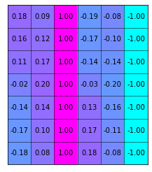
Detailed expression is, note the negative signs in the last 3 columns of data kernel \(\mathbf{G}\):
Practical usage will be introduced later.
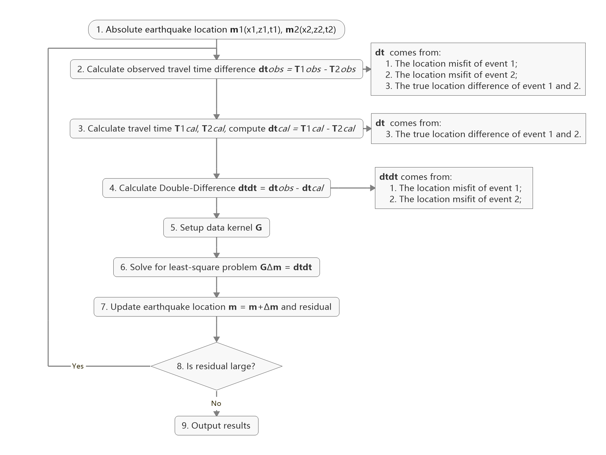
Workflow
hyc1_dd = hyc1_abs.copy()
hyc2_dd = hyc2_abs.copy()
1. Observed Travel Time Difference
obs_trav_t1 = dobs1_delay - hyc1_dd[2] # Travel time = arrival_time - origin_time
obs_trav_t2 = dobs2_delay - hyc2_dd[2]
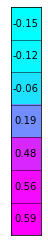
obs_dt = obs_trav_t1 - obs_trav_t2
matrix_show(obs_dt)
2. Calculated Travel Time Difference
dcal1 = np.zeros((nsta,1))
for i in range(dobs1.shape[0]):
    dx = stas[i,0]-hyc1_dd[0]
    dz = stas[i,1]-hyc1_dd[1]
    dcal1[i,0] = np.sqrt(dx**2+dz**2)/Vtrue+hyc1_dd[2]
dcal2 = np.zeros((nsta,1))
for i in range(dobs1.shape[0]):
    dx = stas[i,0]-hyc2_dd[0]
    dz = stas[i,1]-hyc2_dd[1]
    dcal2[i,0] = np.sqrt(dx**2+dz**2)/Vtrue+hyc2_dd[2]
cal_trav_t1 = dcal1 - hyc1_dd[2] # Travel time = calculated_time - origin_time
cal_trav_t2 = dcal2 - hyc2_dd[2]
cal_dt = cal_trav_t1 - cal_trav_t2
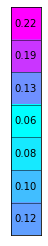
3. Calculate Double-Difference
dtdt = obs_dt - cal_dt
matrix_show(dtdt)
4. Build Up Data Kernel - G
ncol = 3 * 2           # Two event, each has 3 parameter (delta x, delta z, delta t)
G = np.zeros((nsta,ncol))
G[:,2]=1; G[:,5] = -1   # Partial derivative of origin column is 1
for i in range(nsta):
    for j in range(2):
        denomiter1 = np.sqrt((hyc1_dd[0]-stas[i,0])**2+(hyc1_dd[1]-stas[i,1])**2)
        G[i,j]=(hyc1_dd[j]-stas[i,j])/denomiter1/Vtrue
        denomiter2 = np.sqrt((hyc2_dd[0]-stas[i,0])**2+(hyc2_dd[1]-stas[i,1])**2)
        G[i,j+3]=-(hyc2_dd[j]-stas[i,j])/denomiter2/Vtrue
matrix_show(G)
5. Check GTG Inverse Exists
\(G\) is not a square matrix, \(G^TG\) is a squared matrix, we then have:
If the inverse of \(G^TG\) exists (the determinnant != 0, in here we have 10 observations to solve for 4 parameters), then:
GTG = np.matmul(G.T,G)
det = np.linalg.det(GTG)  # Calculate matrix determinant
if det == 0:
    print("Error! The determinant is ZERO!!!")
Error! The determinant is ZERO!!!
6. Add Damp to Matrix
Determinant equals zero means there is no unique solution to the inverse problem, that is, the constraints in data kernel G are not enough to get a result, more constraints is needed. The common method is to add damp to the data kernel.
### Damping the kernel Before damping:
After damping:
\(I\) is an identity matrix, in this case, it should have columns with G, so its dimension is \(6\times6\), here:
### Mathematical Meaning Write new constraints in equation, that is:
What does this mean? It means that the solution SHOULD be zero. As a least square problem solution is a trade-off among equations. The application of damping factor will lead to the solution be small values. \(\lambda\) controls the weight(importance) of damping. A large damp will lead to the solution more close to zero.
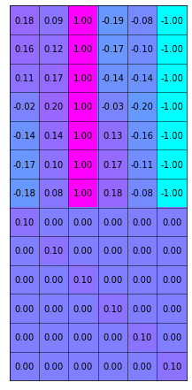
G_dp = np.zeros((nsta+ncol,ncol))
G_dp[:nsta,:] = G
damp = 0.1
G_dp[nsta:,:] = np.diag([1,1,1,1,1,1])*damp
dtdt_damp = np.zeros((nsta+ncol,1))
dtdt_damp[:nsta,0] = dtdt.ravel()
matrix_show(G_dp)
7. Solve Damped Problem
Step 1:
Step 2:
Step 3:
Step 4:
G_dpTG_dp = np.matmul(G_dp.T,G_dp)
G_dpTG_dp_inv = np.linalg.inv(G_dpTG_dp)
G_dpTG_dp_inv_G_dpT = np.matmul(G_dpTG_dp_inv,G_dp.T)
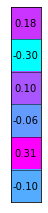
m = np.matmul(G_dpTG_dp_inv_G_dpT,dtdt_damp)
matrix_show(m)
8. Update Location
The output results are the earthquake location misfit with reference to its absolute location. Therefore, the absolute earthquake location should be updated.
hyc1_dd = hyc1_dd+m.ravel()[:3]
hyc2_dd = hyc2_dd+m.ravel()[3:]
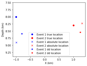
We can see the solutions already depart the initial location and move closer to the true location
xmin = min(hyc1_true[0],hyc1_abs[0],hyc1_dd[0])
xmax = max(hyc1_true[0],hyc1_abs[0],hyc1_dd[0])
ymin = min(hyc1_true[1],hyc1_abs[1],hyc1_dd[1])
ymax = max(hyc1_true[1],hyc1_abs[1],hyc1_dd[1])
plt.plot(hyc1_true[0],hyc1_true[1],"bo",label="Event 1 true location")
plt.plot(hyc2_true[0],hyc2_true[1],"ro",label="Event 2 true location")
plt.plot(hyc1_abs[0],hyc1_abs[1],'bx',label="Event 1 absolute location")
plt.plot(hyc2_abs[0],hyc2_abs[1],'rx',label="Event 2 absolute location")
plt.plot(hyc1_dd[0],hyc1_dd[1],'b*',label="Event 1 dd location")
plt.plot(hyc2_dd[0],hyc2_dd[1],'r*',label="Event 2 dd location")
plt.gca().set_aspect('equal')
plt.legend()
plt.ylim(ymax+0.5,ymin-0.5)
plt.ylabel("Depth (km)")
plt.xlabel("X (km)");
9. Error analysis
The error in observed data will of course lead to uncertainties in the estimation of earthquake location parameters. Their relationship could be described as:
(Wanna know how this relationship derived? Page 435 of An Introduction to Seismology, Earthquakes, and Earth Structure)
mean_dtdt_damp = np.mean(dtdt_damp)
e2 = 0
for i in range(dtdt.shape[0]):
    e2 += (dtdt_damp[i,0] - mean_dtdt_damp)**2
print(f"Square error: ",format(e2,'13.8f'))
var = e2/(dtdt_damp.shape[0]-6)
sigma_m2 = G_dpTG_dp_inv*var
Square error: 0.04330659
present_loc_results(hyc1_dd,sigma_m2[:3,:3])
present_loc_results(hyc2_dd,sigma_m2[3:,3:])
x =   -0.80 ± 0.56  km
z =    8.60 ± 0.64  km
t =   -0.14 ± 0.56  s
x =    1.24 ± 0.55  km
z =    8.54 ± 0.63  km
t =    0.90 ± 0.56  s
Exercise (5 min)
Try to modify the damp parameter and update the results, how it changes? What is the relationship between damping factor, m, and Uncertainty? Can you explain why?
10. Condition Number
We have realized that the damping factor controls the converge rate, a larger damping factor will lead to slow converge rate but small uncertainty; a smaller damping factor will lead to fast converge rate but large uncertainty. Then how to choose proper damping factor?
A good indicator is the conditon number. Conditon number quantifies the relationship between solution error and data error. In earthquake double difference location, the condition number should be in the range 40-100 (empirical).
cond = np.linalg.cond(G_dp)
print("Condtion number is: ",format(cond,'.2f'))
Condtion number is: 37.72
Exercise: Start Another Iteration
The error is still high, update the earthquake location and rerun the process to check the location variation.
Iterative Double-Difference Method
hyc1_loop = hyc1_abs
hyc2_loop = hyc2_abs
niter = 100
k = 0
event_number = 2
event_parameters = 3 #(x,y,z)
#----------Iteration starts----------------------
while k <=niter:
    #----1. Update observed travel time difference------------------
    obs_trav_t1 = dobs1_delay - hyc1_dd[2]               # Travel time = arrival_time - origin_time
    obs_trav_t2 = dobs2_delay - hyc2_dd[2]
    obs_dt = obs_trav_t1 - obs_trav_t2
    #----2. Update calculated travel time difference------------------
    dcal1 = np.zeros((dobs1.shape[0],1))
    for i in range(dobs1.shape[0]):
        dx = stas[i,0]-hyc1_loop[0]
        dz = stas[i,1]-hyc1_loop[1]
        dcal1[i,0] = np.sqrt(dx**2+dz**2)/Vtrue+hyc1_loop[2]
    dcal2 = np.zeros((dobs2.shape[0],1))
    for i in range(dobs1.shape[0]):
        dx = stas[i,0]-hyc2_loop[0]
        dz = stas[i,1]-hyc2_loop[1]
        dcal2[i,0] = np.sqrt(dx**2+dz**2)/Vtrue+hyc2_loop[2]
    cal_trav_t1 = dcal1 - hyc1_dd[2]
    cal_trav_t2 = dcal2 - hyc2_dd[2]
    cal_dt = cal_trav_t1 - cal_trav_t2
    #----3. Calculate double difference-------------------------------
    dtdt = obs_dt - cal_dt
    #----4. Set up G kernel-------------------------------------------
    ncol = event_number * event_parameters
    G = np.zeros((nsta,ncol))
    G[:,2]=1; G[:,5] = -1   # Partial derivative of origin column is 1
    for i in range(nsta):
        for j in range(2):
            denomiter1 = np.sqrt((hyc1_loop[0]-stas[i,0])**2+(hyc1_loop[1]-stas[i,1])**2)
            G[i,j]=(hyc1_loop[j]-stas[i,j])/denomiter1/Vtrue
            denomiter2 = np.sqrt((hyc2_loop[0]-stas[i,0])**2+(hyc2_loop[1]-stas[i,1])**2)
            G[i,j+3]=-(hyc2_loop[j]-stas[i,j])/denomiter2/Vtrue
    #----5. Add damp--------------------------------------------------
    G_dp = np.zeros((nsta+ncol,ncol))
    G_dp[:nsta,:] = G
    damp = 0.1
    G_dp[nsta:,:] = np.diag([1,1,1,1,1,1])*damp
    dtdt_damp = np.zeros((nsta+ncol,1))
    dtdt_damp[:nsta,0] = dtdt.ravel()
    #----6. Solve for Solution-----------------------------------------
    G_dpTG_dp = np.matmul(G_dp.T,G_dp)
    G_dpTG_dp_inv = np.linalg.inv(G_dpTG_dp)
    G_dpTG_dp_inv_G_dpT = np.matmul(G_dpTG_dp_inv,G_dp.T)
    m = np.matmul(G_dpTG_dp_inv_G_dpT,dtdt_damp)
    #----7. Update location-----------------------------------------------
    hyc1_loop = hyc1_loop+m.ravel()[:3]
    hyc2_loop = hyc2_loop+m.ravel()[3:]
    #----8. Error Calculation------------------------------------------------
    mean_dtdt_damp = np.mean(dtdt_damp)
    e2 = 0
    for i in range(dtdt.shape[0]):
        e2 += (dtdt_damp[i,0] - mean_dtdt_damp)**2
    print(f"Iteration {format(k,'4d')} square error: ",format(e2,'13.8f'))
    if e2<0.0000000001:
        print("Itertion stopped for too small error!")
        break
    k = k+1
#--------9. Variance analysis-------------------------------------------
var = e2/(dtdt_damp.shape[0]-event_number * event_parameters)
sigma_m2 = G_dpTG_dp_inv*var
hyc1_dd = hyc1_loop
hyc2_dd = hyc2_loop
Iteration    0 square error:     0.04330659
Iteration    1 square error:     0.00096939
Iteration    2 square error:     0.00013074
Iteration    3 square error:     0.00005316
Iteration    4 square error:     0.00004521
Iteration    5 square error:     0.00004369
Iteration    6 square error:     0.00004278
Iteration    7 square error:     0.00004195
Iteration    8 square error:     0.00004113
Iteration    9 square error:     0.00004032
Iteration   10 square error:     0.00003954
......
Iteration   90 square error:     0.00000830
Iteration   91 square error:     0.00000814
Iteration   92 square error:     0.00000799
Iteration   93 square error:     0.00000784
Iteration   94 square error:     0.00000769
Iteration   95 square error:     0.00000754
Iteration   96 square error:     0.00000740
Iteration   97 square error:     0.00000726
Iteration   98 square error:     0.00000713
Iteration   99 square error:     0.00000699
Iteration  100 square error:     0.00000686
present_loc_results(hyc1_dd,sigma_m2[:3,:3],std_fmt='.5f')
present_loc_results(hyc2_dd,sigma_m2[3:,3:],std_fmt='.5f')
x =   -0.87 ± 0.00700  km
z =    8.16 ± 0.00790  km
t =   -0.12 ± 0.00700  s
x =    1.14 ± 0.00700  km
z =    8.41 ± 0.00800  km
t =    0.88 ± 0.00700  s
LSQR Algorithm
Considering a double difference cluster with 1000 events, we estimate the time consumed for one iteration. Note the \(G^TG\) dimension is \(4000\times 4000\), it costs 16 seconds to calculate the inverse and singular value decomposition. What about 10 k events?
G = np.random.randn(4000,4000)
tmp1 = time.time()
G_inv = np.linalg.inv(G)
u,s,vt = np.linalg.svd(G_inv)
tmp2 = time.time()
print(tmp2-tmp1,' s')
if (tmp2-tmp1)>5:
    print("Wow, it cost a lot of time of do the calculation")
38.39115285873413  s
Wow, it cost a lot of time of do the calculation
Introduction to LSQR
Least-Square QR decompositon (LSQR, Paige, C.C and Saunders, M.A. (1982)) method is developed for least-square solution for large dataset, its performance in ill-conditioned problems is superior.
From problem \(\mathbf{Am=b}\), \(\mathbf{A}\) maps the solution to the data space. \(\mathbf{A^T}\) maps the data to the solution space. LSQR method eliminates residual iteratively with limited computation.
To ensure the stability of method, each A column is required to be scaled up to be unit value. That is:
After get the solution, a conversion between \(\mathbf{m'}\) and \(\mathbf{m}\) is needed by \(m_i=\frac{m'_i}{\|A_i\|}\)
hyc1_loop = hyc1_abs
hyc2_loop = hyc2_abs
niter = 100
k = 0
event_number = 2
event_parameters = 3 #(x,y,z)
#----------Iteration starts----------------------
while k <=niter:
    #----1. Update observed travel time difference------------------
    obs_trav_t1 = dobs1_delay - hyc1_dd[2]               # Travel time = arrival_time - origin_time
    obs_trav_t2 = dobs2_delay - hyc2_dd[2]
    obs_dt = obs_trav_t1 - obs_trav_t2
    #----2. Update calculated travel time difference------------------
    dcal1 = np.zeros((dobs1.shape[0],1))
    for i in range(dobs1.shape[0]):
        dx = stas[i,0]-hyc1_loop[0]
        dz = stas[i,1]-hyc1_loop[1]
        dcal1[i,0] = np.sqrt(dx**2+dz**2)/Vtrue+hyc1_loop[2]
    dcal2 = np.zeros((dobs2.shape[0],1))
    for i in range(dobs1.shape[0]):
        dx = stas[i,0]-hyc2_loop[0]
        dz = stas[i,1]-hyc2_loop[1]
        dcal2[i,0] = np.sqrt(dx**2+dz**2)/Vtrue+hyc2_loop[2]
    cal_trav_t1 = dcal1 - hyc1_dd[2]
    cal_trav_t2 = dcal2 - hyc2_dd[2]
    cal_dt = cal_trav_t1 - cal_trav_t2
    #----3. Calculate double difference-------------------------------
    dtdt = obs_dt - cal_dt
    #----4. Set up G kernel-------------------------------------------
    ncol = event_number * event_parameters
    G = np.zeros((nsta,ncol))
    G[:,2]=1; G[:,5] = -1   # Partial derivative of origin column is 1
    for i in range(nsta):
        for j in range(2):
            denomiter1 = np.sqrt((hyc1_loop[0]-stas[i,0])**2+(hyc1_loop[1]-stas[i,1])**2)
            G[i,j]=(hyc1_loop[j]-stas[i,j])/denomiter1/Vtrue
            denomiter2 = np.sqrt((hyc2_loop[0]-stas[i,0])**2+(hyc2_loop[1]-stas[i,1])**2)
            G[i,j+3]=-(hyc2_loop[j]-stas[i,j])/denomiter2/Vtrue
    #---- Scale up G columns to unit length--------------------------
    Gnorms = np.zeros(ncol)
    for i in range(ncol):
        norm = np.linalg.norm(G[:,i])
        Gnorms[i] = norm
        G[:,i] = G[:,i]/norm
    #----6. LSQR and rescale solution---------------------------------
    damp = 0.1
    A = csc_matrix(G, dtype=float)
    m,istop,itn,r1norm,r2norm,anorm,acond,arnorm,xnorm,var=lsqr(A,dtdt,damp=damp,calc_var=True)
    m = np.divide(m,Gnorms)
    var = np.divide(var,Gnorms**2)
    #----7. Update location-----------------------------------------------
    hyc1_loop = hyc1_loop+m.ravel()[:3]
    hyc2_loop = hyc2_loop+m.ravel()[3:]
    #----8. Error Calculation------------------------------------------------
    print(f"Iteration {format(k,'4d')} residual: ",format(r1norm,'13.8f'))
    if r1norm<0.0000000001:
        print("Itertion stopped for too small error!")
        break
    k = k+1
#--------9. Variance analysis-------------------------------------------
sigma_m2 = np.diag(var)**2*r2norm**2
hyc1_dd = hyc1_loop
hyc2_dd = hyc2_loop
Iteration    0 residual:     0.01522528
Iteration    1 residual:     0.00683196
Iteration    2 residual:     0.00624882
Iteration    3 residual:     0.00581534
Iteration    4 residual:     0.00541587
Iteration    5 residual:     0.00504727
Iteration    6 residual:     0.00470742
Iteration    7 residual:     0.00439429
Iteration    8 residual:     0.00410597
Iteration    9 residual:     0.00384061
Iteration   10 residual:     0.00359645
......
Iteration   95 residual:     0.00013054
Iteration   96 residual:     0.00012620
Iteration   97 residual:     0.00012201
Iteration   98 residual:     0.00011796
Iteration   99 residual:     0.00011405
Iteration  100 residual:     0.00011026
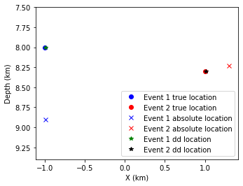
We then find the residual is very small, and the earthquake location almost reached its true location
xmin = min(hyc1_true[0],hyc1_abs[0],hyc1_dd[0])
xmax = max(hyc1_true[0],hyc1_abs[0],hyc1_dd[0])
ymin = min(hyc1_true[1],hyc1_abs[1],hyc1_dd[1])
ymax = max(hyc1_true[1],hyc1_abs[1],hyc1_dd[1])
plt.plot(hyc1_true[0],hyc1_true[1],"bo",label="Event 1 true location")
plt.plot(hyc2_true[0],hyc2_true[1],"ro",label="Event 2 true location")
plt.plot(hyc1_abs[0],hyc1_abs[1],'bx',label="Event 1 absolute location")
plt.plot(hyc2_abs[0],hyc2_abs[1],'rx',label="Event 2 absolute location")
plt.plot(hyc1_dd[0],hyc1_dd[1],'*',color='green',label="Event 1 dd location")
plt.plot(hyc2_dd[0],hyc2_dd[1],'*',color='k',label="Event 2 dd location")
plt.gca().set_aspect('equal')
plt.legend()

plt.ylim(ymax+0.5,ymin-0.5)
plt.ylabel("Depth (km)")
plt.xlabel("X (km)");
present_loc_results(hyc1_dd,sigma_m2[:3,:3],std_fmt='.8f')
present_loc_results(hyc2_dd,sigma_m2[3:,3:],std_fmt='.8f')
x =   -0.99 ± 0.03210000  km
z =    8.00 ± 0.04610000  km
t =   -0.12 ± 0.00000000  s
x =    1.01 ± 0.03280000  km
z =    8.30 ± 0.04760000  km
t =    0.88 ± 0.00000000  s
Summary
In this tutorial, we first demonstrate the influence of velocity misfit and Station delay’s influence on earthquake location results.
We then introduce the double-difference method, which theoretically diminishes the station delay effect and limits the influence of velocity misfit. During processing, we: * Set up the data kernel G and calculate the double difference array dtdt * Add damping to the data kernel to make it stable (determinant not be zero) * Use conditon number to guide the selection of damping factor * Comparison shows double-difference location leads to location with better performance
Note
Homework
In the demo example, is event origin time fully recovered? Could you please explain the reason?(10 points)
Note we add negative symbol to partial derivatives of the event 2 in constructing the data kernel, do you know why? (10 points)
In calculating the variance(var), it is written
var = e2/(dtdt_damp.shape[0]-event_number * event_parameters), do you know why variance is different from square error here? (10 points)Add one more event hyc_true3 = (0.2,8.1,1) (x,z,t) and prepare for inversion, set up suitable damping factor so that condition number is in the range 40-100.(80 points) - Show the absolute location result of the newly added event and its uncertainty. (20 points) - Show your data kernel G for Double-Difference inversion and its determinant. (20 points) - Show your Double-Difference inversion result and its uncertainty, how many iterations you used? (20 points) - Did your results get closer to true earthquake locations? Make a plot and show (20 points) #### Hint The dimension of \(m\) should be \(9 \times 1\)
\[m^T = \begin{bmatrix} \Delta x_1&\Delta z_1&\Delta t_1 & \Delta x_2&\Delta z_2&\Delta t_2 & \Delta x_3&\Delta z_3&\Delta t_3 \end{bmatrix}\]For the double-difference value of event_1 and event_2 recorded in station k, its corresponding row of data kernel G should be:
\[\begin{bmatrix} \frac{\partial T^{1}_{k}}{\partial x}&\frac{\partial T^{1}_{k}}{\partial z}&\frac{\partial T^{1}_{k}}{\partial t}& -\frac{\partial T^{2}_{k}}{\partial x}&-\frac{\partial T^{2}_{k}}{\partial z}&-\frac{\partial T^{2}_{k}}{\partial t}& 0&0&0 \end{bmatrix}\]For the double-difference value of event_2 and event_3 recorded in station k, its corresponding row of data kernel G should be:
\[\begin{bmatrix} 0&0&0& \frac{\partial T^{2}_{k}}{\partial x}&\frac{\partial T^{2}_{k}}{\partial z}&\frac{\partial T^{2}_{k}}{\partial t}& -\frac{\partial T^{3}_{k}}{\partial x}&-\frac{\partial T^{3}_{k}}{\partial z}&-\frac{\partial T^{3}_{k}}{\partial t} \end{bmatrix}\]
Source code
Download tutorial code here