Generic Mapping Tools - Seismic Data
Plotting earthquake catalog
Preview
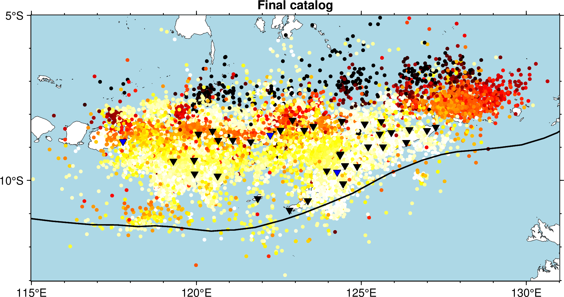
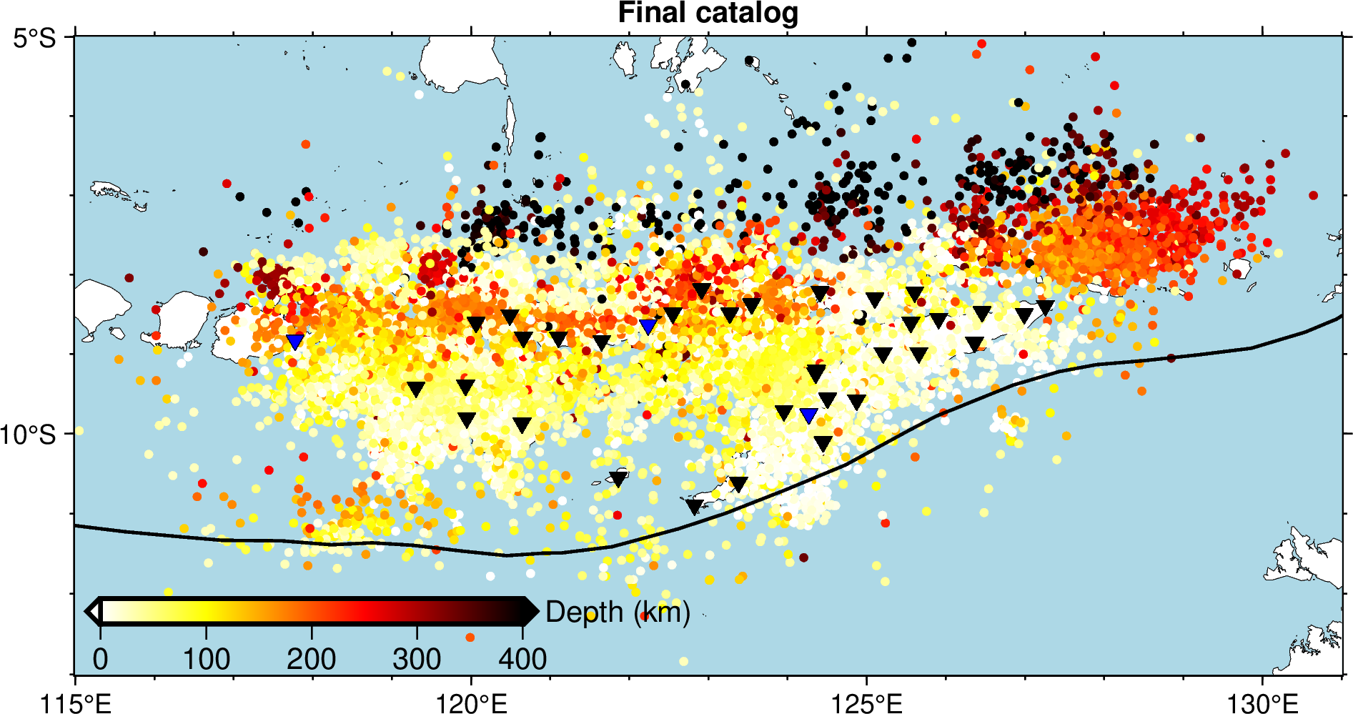
The figure below is modified from Figure 2 in this paper.
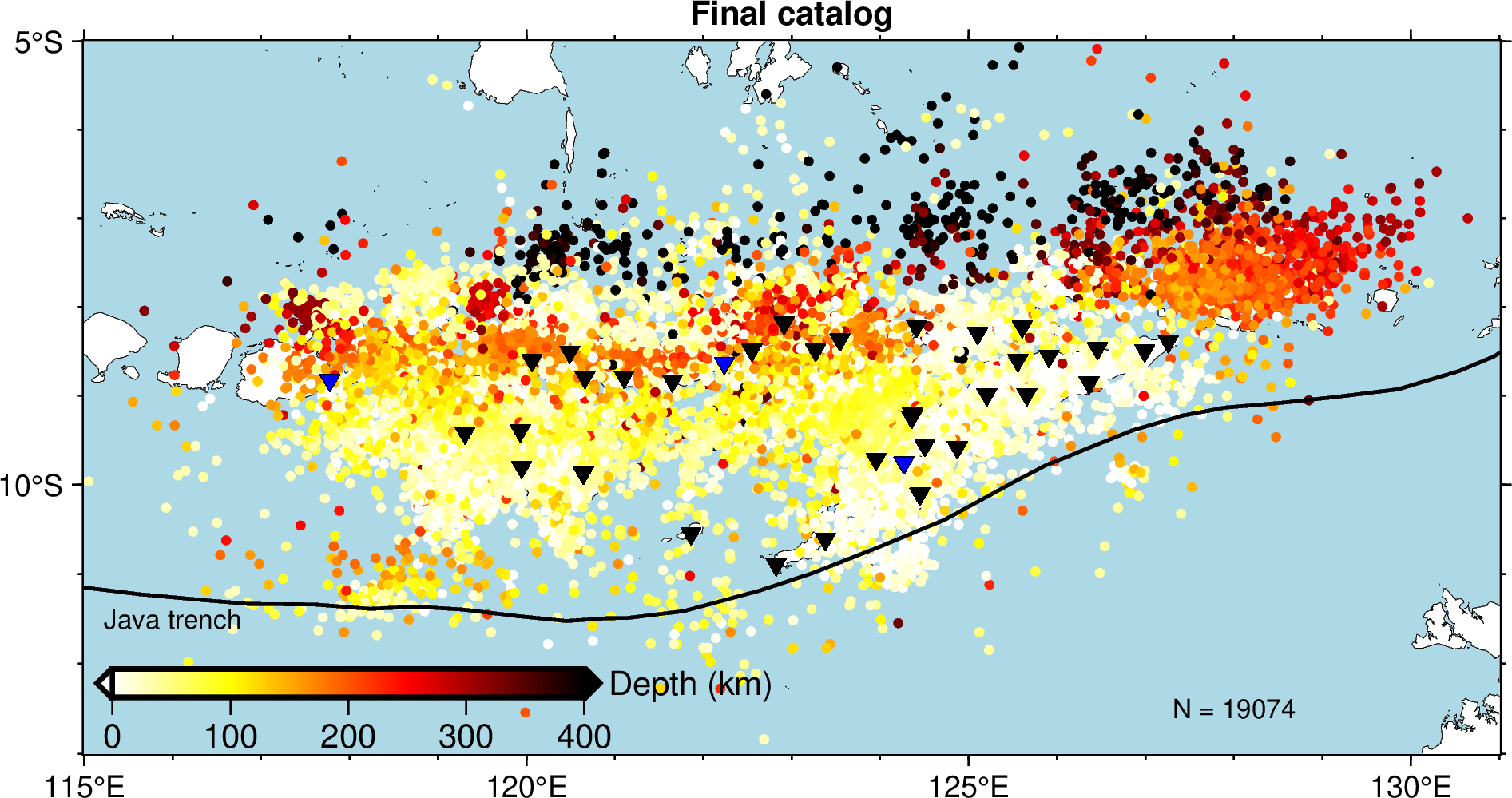
It is generated using the following commands:
#!/bin/sh
gmt begin catalog png
# the frame
gmt basemap -JM15c -R115/131/-13/-5 -Bxa5f1 -Bya5f1 -BWeSn+t"Final catalog" --MAP_FRAME_TYPE=plain --FONT_TITLE=10p --MAP_TITLE_OFFSET=-8p
# plotting coastline with specify land and sea colours
gmt coast -Gwhite -Slightblue -W0.1p,black -Da
# creating customized colormaps
gmt makecpt -Chot -T0/400/10 -D -Z -Ic -H > depth.cpt
awk '{print $9,$8,$10}' banda_arc_catalog.txt > catalog.xyz

# plotting the earthquake data
gmt plot catalog.xyz -Sc0.1c -Cdepth.cpt
# plotting the trench
gmt plot java_trench.txt -W1p,black
# extracting station data and plot them
awk 'NR>1 {print $5,$6}' GE_3_stations.txt |gmt psxy -Si7p -W0.01p,black -Gblue
awk -F"|" 'NR>3 {print $6,$5}' YS_30_stations.txt |gmt psxy -Si7p -W0.01p,black -Gblack
# creating a colorbar
gmt colorbar -DjBL+h+o0.3c/0.6c+jBL+w5c/0.3c+e -By+l"Depth (km)" -Bxa100 -Cdepth.cpt
# plotting text
echo "128 -12.5 N = 19074" | gmt text -F+f8p,black
echo "116 -11.5 Java trench" | gmt text -F+f8p,black
gmt end
To reproduce it by yourself, you may first download or save banda_arc_catalog.txt, java_trench.txt, GE_3_stations.txt, YS_30_stations.txt, and then move these files into your working directory. Try to copy the above commands and run them on your own computer to see if you can generate the same figure without warning or error.
Step-by-Step explanation
-JM15c specifies the map projection type to be Mercator projection. The width of map is 15c (15 centimeters).
-R115/131/-13/-5 specifies the map range, minimum and maximum longitudes are 115 and 131, minimum and maximum latitudes are -13 -5.
-Bxa5f1 specifies that x axes have ticklabels with interval of 5 and ticks with interval of 1.
-Bya5f1 specifies that y axes have ticklabels with interval of 5 and ticks with interval of 1.
-BWeSn+t"Final catalog" specifies that the left and bottom ticklabels are visible, which the right and top ticklabels are invisible, where the +t"Final catalog" indicates plotting the title “Final catalog”
--MAP_FRAME_TYPE=plain --FONT_TITLE=10p --MAP_TITLE_OFFSET=-8p are the gmt settings. --MAP_FRAME_TYPE=plain specifies the frame type as plain(i.e., simple line); --FONT_TITLE=10p specifies the font of title to be 10p; --MAP_TITLE_OFFSET=-8p specifies the distance between the title with the frame to be -8p.
-Gwhite specifies fill the dry/land area with white.
-Slightblue specifies fill the wet/sea/lake area with lightblue.
--W0.1p,black specifies the line with a witdh of 0.1p and line color of black.
-Da specifies automatically selects the appropriate data precision based on the size of the current drawing area
-Chot specifies the input cpt used is hot
-D selects the back- and foreground colors for the colorbar
-Z creates a continuous cpt file
-Ic reverse the CPT
catalog.xyz contains three columns of data. longitude, latitude, and depth. The value of depth column will be used for coloring points based on CPT file.
-DjBL+h+o0.3c/0.6c+jBL+w5c/0.3c+e specifices the paramter of colorbar. -DjBL means plot color at the Bottom Left; +h means
draw horizontal color scale; +o0.3c/0.6c means plot move the colorbar 0.3 cm in X direction and 0.6 cm in Y Direction; +w5c/0.3c means plot a colorbar with a length of 5 cm and a width of 0.3 cm; +e means add a triangle to the foreground and background colors in the colorbar.
-F+f8p,black specifices the font size of 8p and color of black
Plotting cross sections
Preview
The figure below is modified from Figure 3 in this paper.
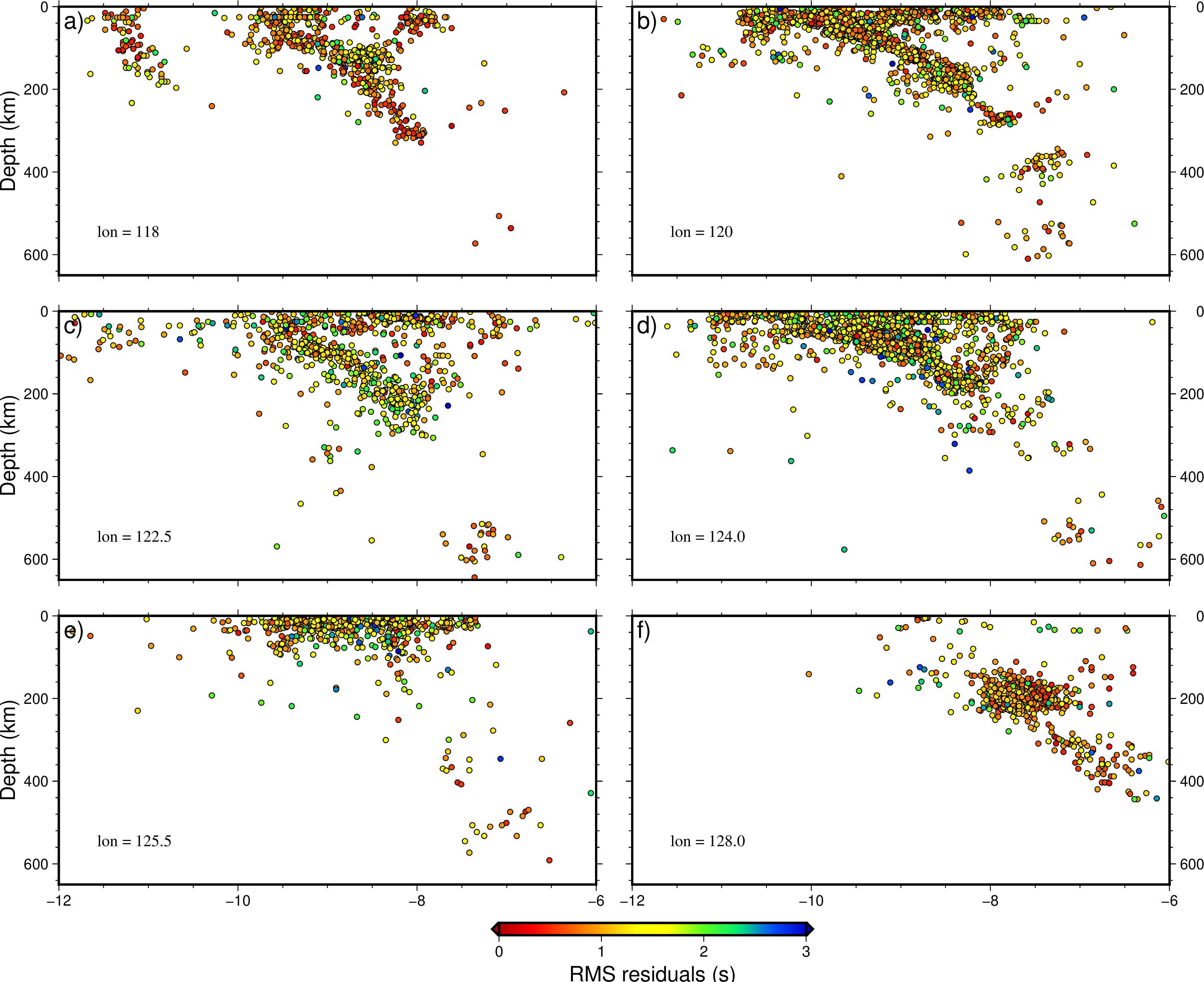
It is generated using the following commands:
#!/bin/sh
# extract data ignoring header, in order : lon, lat, depth, residual
awk 'NR>1 {print $9,$8,$10,$7}' banda_arc_catalog.txt > extracted.txt

gmt begin section png
gmt makecpt -Cseis -T0/3/0.1 -D -Z -H > res.cpt

gmt subplot begin 3x2 -Fs14c/7c -A
gmt subplot set 0 # transect along lon = 118
# project the data within 0.5 degree onto plane
# output file in order: latitude , depth , residual
gmt project extracted.txt -C118/-12 -E118/-6 -Lw -W-0.5/0.5 -Fyz > projected_input.txt
gmt plot projected_input.txt -JX14c/-7c -R-12/-6/0/650 -BWesn -Bya200f40+l"Depth (km)" -Bxa2f0.5 -Sc4p -W0.5p -Cres.cpt # ploting
echo "lon = 118" | gmt text -F+cBL+f12p,4,black -Dj1c/1c # adding text

gmt subplot set 1 # transect along lon = 120
# project the data within 0.5 degree onto plane
# output file in order: latitude , depth , residual
gmt project extracted.txt -C120/-12 -E120/-6 -Lw -W-0.5/0.5 -Fyz > projected_input.txt
gmt plot projected_input.txt -JX14c/-7c -R-12/-6/0/650 -BwEsn -Bya200f40 -Bxa2f0.5 -Sc4p -W0.5p -Cres.cpt # ploting
echo "lon = 120" | gmt text -F+cBL+f12p,4,black -Dj1c/1c # adding text

gmt subplot set 2 # transect along lon = 122.5
# project the data within 0.5 degree onto plane
# output file in order: latitude , depth , residual
gmt project extracted.txt -C122.5/-12 -E122.5/-6 -Lw -W-0.5/0.5 -Fyz > projected_input.txt
gmt plot projected_input.txt -JX14c/-7c -R-12/-6/0/650 -BWesn -Bya200f40+l"Depth (km)" -Bxa2f0.5 -Sc4p -W0.5p -Cres.cpt # ploting
echo "lon = 122.5" | gmt text -F+cBL+f12p,4,black -Dj1c/1c # adding text

gmt subplot set 3 # transect along lon = 124.0
# project the data within 0.5 degree onto plane
# output file in order: latitude , depth , residual
gmt project extracted.txt -C124.0/-12 -E124.0/-6 -Lw -W-0.5/0.5 -Fyz > projected_input.txt
gmt plot projected_input.txt -JX14c/-7c -R-12/-6/0/650 -BwEsn -Bya200f40 -Bxa2f0.5 -Sc4p -W0.5p -Cres.cpt # ploting
echo "lon = 124.0" | gmt text -F+cBL+f12p,4,black -Dj1c/1c # adding text

gmt subplot set 4 # transect along lon = 125.5
# project the data within 0.5 degree onto plane
# output file in order: latitude , depth , residual
gmt project extracted.txt -C125.5/-12 -E125.5/-6 -Lw -W-0.5/0.5 -Fyz > projected_input.txt
gmt plot projected_input.txt -JX14c/-7c -R-12/-6/0/650 -BWeSn -Bya200f40+l"Depth (km)" -Bxa2f0.5 -Sc4p -W0.5p -Cres.cpt # ploting
echo "lon = 125.5" | gmt text -F+cBL+f12p,4,black -Dj1c/1c # adding text

gmt subplot set 5 # transect along lon = 128.0
# project the data within 0.5 degree onto plane
# output file in order: latitude , depth , residual
gmt project extracted.txt -C128.0/-12 -E128.0/-6 -Lw -W-0.5/0.5 -Fyz > projected_input.txt
gmt plot projected_input.txt -JX14c/-7c -R-12/-6/0/650 -BwESn -Bya200f40 -Bxa2f0.5 -Sc4p -W0.5p -Cres.cpt # ploting
echo "lon = 128.0" | gmt text -F+cBL+f12p,4,black -Dj1c/1c # adding text

gmt subplot end

gmt colorbar -DJBC+e+w8c+o1c -Cres.cpt -Bxa1+L"RMS residuals (s)"
gmt end
To reproduce it by yourself, you may first download or save banda_arc_catalog.txt and then move this files into your working directory. Try to copy the above commands and run them on your own computer to see if you can generate the same figure without warning or error.
You may go to the official tutorial website of GMT v6.3 for more exploring
Excercises
Reproduce figure 1 in the paper
include the base map and other samples (including the station, plate boundary, subduct direction arrows, and so on)
plot the station name, filled the station samples by yellow, and the station list in Unix command by red.
add a scale to the figure.
plot the map view cross-section, mark two ends of it with “A” and “A’”. The cross-section should cross through the “MMRI” station, and with a length of 300 km, strike 30 degrees west of north
Plot a cross-section plot based on the catalog generated in the Unix command tutorial
project the earthquake within 30 km to the cross-section.
Scale the circles by earthquake magnitude and filled the circle according to their depth.
marked “A” and “A’” in the figure.
Plot the magnitude variation figure. Refer to Figure 4b in the paper
used stars to represent 10 maximum magnitude earthquakes. and label the magnitude of the largest one.
filled the circle according to their depth.