Generic Mapping Tools
Brief introduction
What is GMT?
The Generic Mapping Tools (GMT) is one of the most popular mapping softwares in the world;
It is widely used across the Earth, Ocean, and Planetary sciences and beyond;
It is a free, open source software licensed under the GNU LGPL license.

What can GMT do?
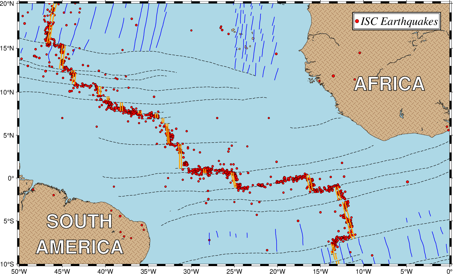
How to install GMT?
Note
The following steps have been tested successfully for Linux, macOS, and window subsystem for linux.
Warning
Exclude $ and start without whitespace!
$ conda create --name gmt-env
$ conda activate gmt-env
$ conda install gmt -c conda-forge
$ gmt --version
6.3.0
Start with three simple examples
$ gmt coast -Rg -JH15c -Gpurple -Baf -B+t"My First Plot" -pdf,png GlobalMap1
$ gmt begin GlobalMap2 png,pdf
$ gmt coast -Rg -JH15c -Gpurple -Baf -B+t"My Second Plot"
$ gmt end show
$ cat GlobalMap3.sh
#!/bin/sh
gmt begin GlobalMap3 png,pdf
gmt coast -Rg -JH15c -Gpurple -Baf -B+t"My Third Plot"
gmt end show
$ sh GlobalMap3.sh
No difference found! And do you think which way is better, especially for very complex figures? There is no doubt that the third way, (i..e., based on script), is better. Since we can simply modify the script and re-run the script to refine the figure.
Basic structure of GMT script
Now let’s take a further look at the third example in the previous part
#!/bin/sh specifies sh as the command language interpreter.Tip
#!/bin/sh by #!/dir/to/shgmt begin GlobalMap3 png,pdf initiates a new GMT session. The output figure name is GlobalMap3. The output figure format are png and pdf.Note
gmt coast -Rg -JH15c -Gpurple -Baf -B+t"My Third Plot" adds the first layer. If it’s followed by other commands, as shown in later parts, this layer will be overlaid by new layers.Note
gmt end show terminates the GMT session. If show exists, the produced figure of the first format will be opened by default viewer.There are a lot of GMT commands and much much much more options. Here, this tutorial aims to give GMT beginners very quick training. Therefore, we will show readers how to generate figures from public seismic data using some commonly used commands. More specificlly, It includes: 1. Plotting topographic map 2. Plotting earthquake catalog 3. Plotting cross sections.
Plotting topographic map
Preview
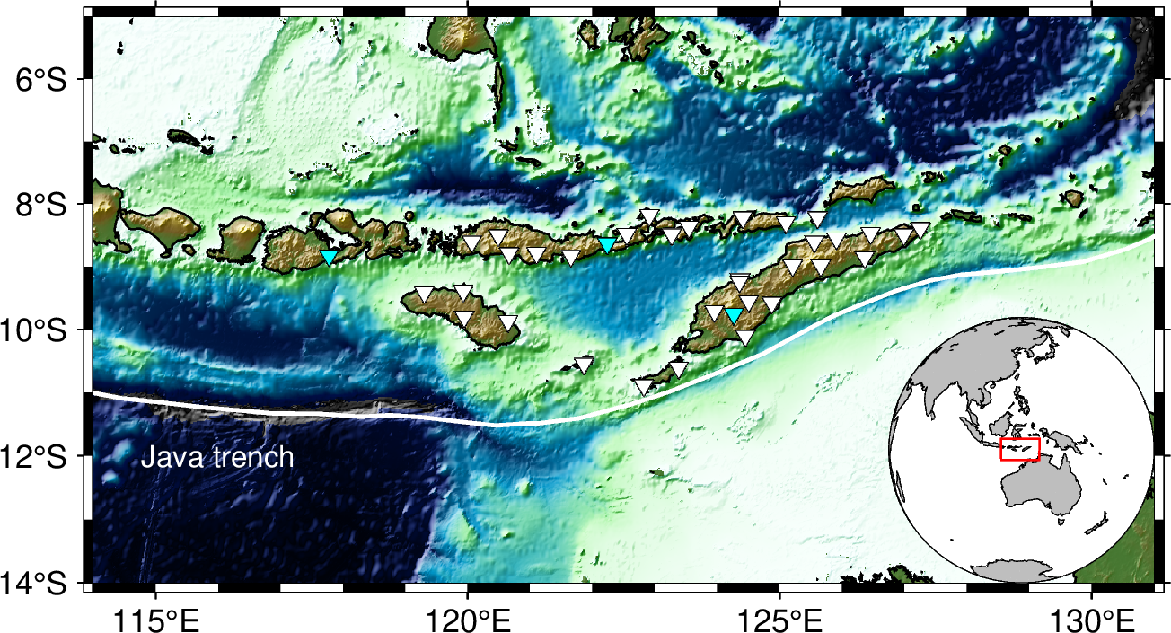
After learning this part, you will be able to create the figure below or similar ones.
The figure below is modified from Figure 1 in this paper.

It is generated using the following commands:
#!/bin/sh

gmt begin Banda_Arc_Region png

# constructing the frame
gmt basemap -JM10c -R114/131/-14/-5 -BWeSn -Bxa5f1 -Bya2f1
# creating a colormap with customized boundaries
gmt makecpt -Crelief -T-6000/6000/200 -D -Z -H > elevation.cpt
# plotting the topography data, which can be remotely obtained from gmt database using the @earth_relief_??? option
gmt grdimage @earth_relief_01m -Celevation.cpt -I+
# plotting the coastline data
gmt coast -W0.5p,black -Da
# inset a global figure with the specify boundary
gmt inset begin -Dn1/0+jBR+w2.5c
gmt coast -Rg -JG123/-10/90/? -B -Swhite -A5000 -Ggray -W0.2p,black -Da --MAP_FRAME_PEN=0.2p
echo -e "\n114 -14\n131 -14\n131 -5\n114 -5\n114 -14" | gmt plot -W0.5p,red
gmt inset end
# plotting the trench data using given data file
gmt plot java_trench.txt -W1p,white
# inserting text
echo '116 -12 Java trench' | gmt text -F+f8p,white
# extracting stations locations from data files
awk 'NR>1 {print $5,$6}' GE_3_stations.txt | gmt plot -Si6p -W0.1p,black -Gcyan
awk -F"|" 'NR>3 {print $6,$5}' YS_30_stations.txt | gmt plot -Si6p -W0.1p,black -Gwhite
# creating colorbar legend
gmt colorbar -Dn1/0+o0.5c/0c+jBL+w5.5c -Bxa3000 -By+l"Topo (m)" -Celevation.cpt

gmt end show

rm elevation.cpt
To reproduce it by yourself, you may first download or save java_trench.txt, GE_3_stations.txt, YS_30_stations.txt, and then move these files into your working directory. Try to copy the above commands and run them on your own computer to see if you can generate the same figure without warning or error.
Step-by-Step explanation
-JM10c specifies the map projection type to be Mercator projection. The width of map is 10c (10 centimeters).
-R114/131/-14/-5 specifies the map range, minimum and maximum longitudes are 114 and 131, minimum and maximum latitudes are -14 -5.
-BWeSn specifies that the left and bottom ticklabels are visible, which the right and top ticklabels are invisible.
-Bxa5f1 specifies that x axes have ticklabels with interval of 5 and ticks with interval of 1.
-Bya2f1 specifies that y axes have ticklabels with interval of 2 and ticks with interval of 1.

-Crelief specifies the input cpt to be relief, click to see a full list of built-in cpt

-T-6000/6000/200 defines the range of the new CPT by giving the lowest and highest z-values as -6000 and 6000, the increment is 200.
-D selects the back- and foreground colors to match the colors for lowest and highest z-values in the output CPT.
-Z forces a continuous CPT when building from a list of colors and a list of z-values [discrete].
-H is required for modern mode.
> elevation.cpt save the output CPT into a file named elevation.cpt
@earth_relief_01m will download global relief grids (the resolution is 1 minute, it depends on the map range) from the GMT server. Click to view a full list of provided Global Relief Datasets
-Celevation.cpt specifies which CPT to use.
-I+ selects the default arguments to apply intensity.

-W0.5p,black specifies the line width to be 0.5p (0.5 point) and line color to be black.
-Da means that selecting the resolution of shorelines automaticly.
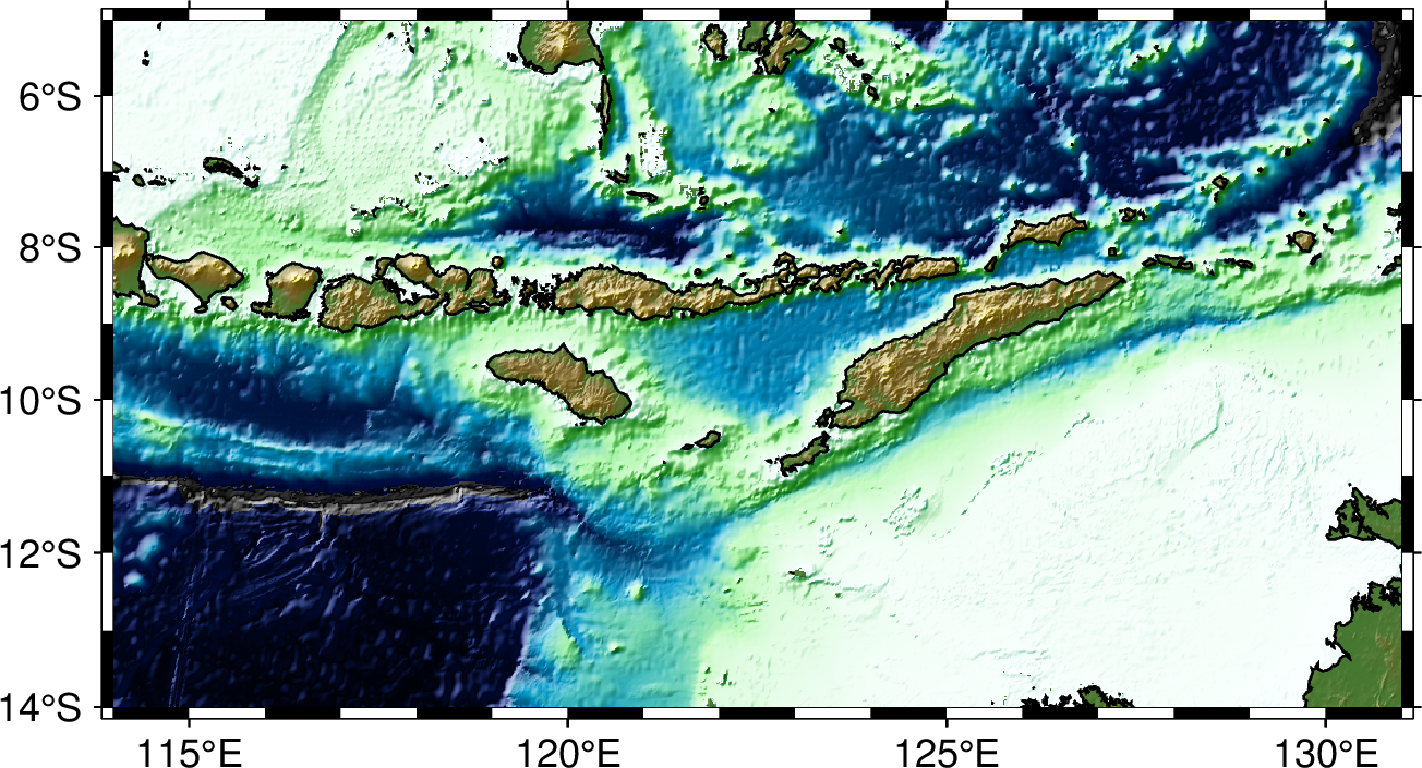
-Dn1/0+jBR+w2.5c gives the location and size of the inset. Now the anchor point is relative to both main and inset map. In the main map, both x and y axes are normalzied with range to be 0-1. So here n1/0 means the right most and lower most point, i.e., the bottom right point of the main map. In the inset map, the location of this anchor point is also at bottom right (BR). And the width of the inset map is 2.5c.
-Rg specifies the global domain.
-JG123/-10/90/? specifies the projection type to be orthographic azimuthal projection and the center longitude and latitude to be 123 and -10. The horizon is 90 degree (<=90). The width is same as the inset map, thus use ?.
-B means no ticks and gridlines.
-Swhite specifies the color of wet areas to be white.
-A5000 means that an area smaller than 5000 km^2 will not be plotted.
-Ggray specifies the color of dry areas to be gray.
--MAP_FRAME_PEN=0.2p sets the map’s frame width to be 0.2p.
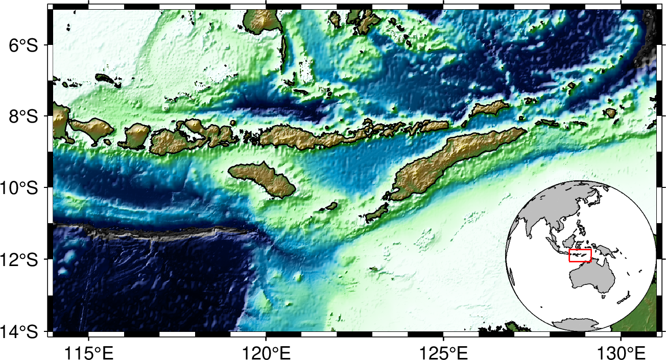
java_trench.txt contains two columns of data, the first column is longitude and the second column is latitude. Each row means a sample point along the trench line.
-W1p,white specifies the line width and color to be 1p and white.
116 -12 specifies the location.
Java trench is the text being added.
-F+f8p,white specfies the fontsize and color of text.
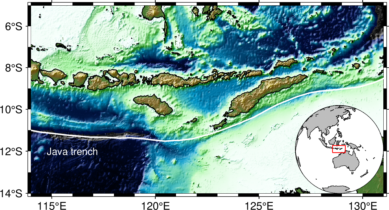
Si6p specifies the symbols to be inverted triangles (i) and their size is 6p.
-Gcyan specifies fill color of the symbols.
-W0.1p,black specifies the outline properties of symbols.
+o0.5c/0c means the anchor point in the main figure is further moved for 0.5c along the x direction.
-By+l"Topo (m)" adds a label along the y axis.
Plotting earthquake catalog
Preview
The figure below is modified from Figure 2 in this paper.
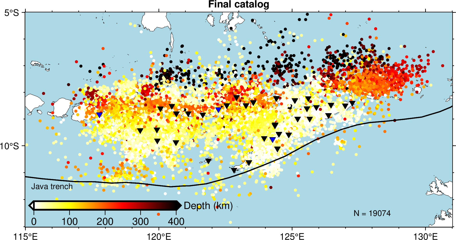
It is generated using the following commands:
#!/bin/sh
gmt begin catalog png
# the frame
gmt basemap -JM15c -R115/131/-13/-5 -Bxa5f1 -Bya5f1 -BWeSn+t"Final catalog" --MAP_FRAME_TYPE=plain --FONT_TITLE=10p --MAP_TITLE_OFFSET=-8p
# plotting coastline with specify land and sea colours
gmt coast -Gwhite -Slightblue -W0.1p,black -Da
# creating customized colormaps
gmt makecpt -Chot -T0/400/10 -D -Z -Ic -H > depth.cpt
awk '{print $9,$8,$10}' banda_arc_catalog.txt > catalog.xyz

# plotting the earthquake data
gmt plot catalog.xyz -Sc0.1c -Cdepth.cpt
# plotting the trench
gmt plot java_trench.txt -W1p,black
# extracting station data and plot them
awk 'NR>1 {print $5,$6}' GE_3_stations.txt |gmt psxy -Si7p -W0.01p,black -Gblue
awk -F"|" 'NR>3 {print $6,$5}' YS_30_stations.txt |gmt psxy -Si7p -W0.01p,black -Gblack
# creating a colorbar
gmt colorbar -DjBL+h+o0.3c/0.6c+jBL+w5c/0.3c+e -By+l"Depth (km)" -Bxa100 -Cdepth.cpt
# plotting text
echo "128 -12.5 N = 19074" | gmt text -F+f8p,black
echo "116 -11.5 Java trench" | gmt text -F+f8p,black
gmt end
To reproduce it by yourself, you may first download or save banda_arc_catalog.txt, java_trench.txt, GE_3_stations.txt, YS_30_stations.txt, and then move these files into your working directory. Try to copy the above commands and run them on your own computer to see if you can generate the same figure without warning or error.
Step-by-Step explanation
-JM15c specifies the map projection type to be Mercator projection. The width of map is 15c (15 centimeters).
-R115/131/-13/-5 specifies the map range, minimum and maximum longitudes are 115 and 131, minimum and maximum latitudes are -13 -5.
-Bxa5f1 specifies that x axes have ticklabels with interval of 5 and ticks with interval of 1.
-Bya5f1 specifies that y axes have ticklabels with interval of 5 and ticks with interval of 1.
-BWeSn+t"Final catalog" specifies that the left and bottom ticklabels are visible, which the right and top ticklabels are invisible, where the +t"Final catalog" indicates plotting the title “Final catalog”
--MAP_FRAME_TYPE=plain --FONT_TITLE=10p --MAP_TITLE_OFFSET=-8p are the gmt settings. --MAP_FRAME_TYPE=plain specifies the frame type as plain(i.e., simple line); --FONT_TITLE=10p specifies the font of title to be 10p; --MAP_TITLE_OFFSET=-8p specifies the distance between the title with the frame to be -8p.

-Gwhite specifies fill the dry/land area with white.
-Slightblue specifies fill the wet/sea/lake area with lightblue.
--W0.1p,black specifies the line with a witdh of 0.1p and line color of black.
-Da specifies automatically selects the appropriate data precision based on the size of the current drawing area

-Chot specifies the input cpt used is hot

-Ic reverse the CPT
catalog.xyz contains three columns of data. longitude, latitude, and depth. The value of depth column will be used for coloring points based on CPT file.
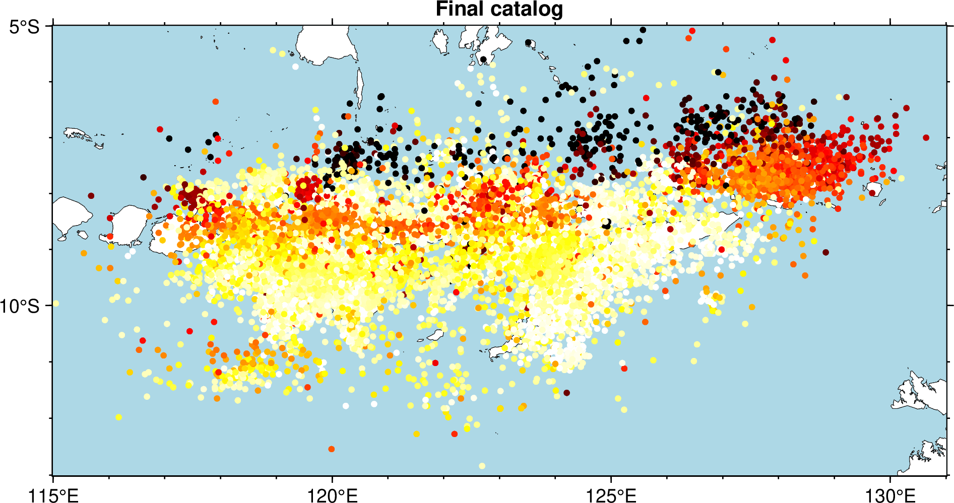
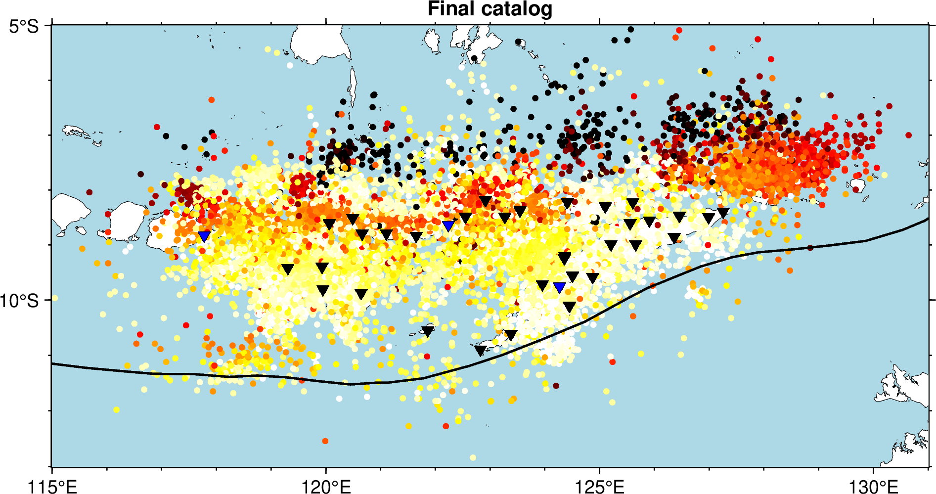
-DjBL+h+o0.3c/0.6c+jBL+w5c/0.3c+e specifices the paramter of colorbar. -DjBL means plot color at the Bottom Left; +h means
draw horizontal color scale; +o0.3c/0.6c means plot move the colorbar 0.3 cm in X direction and 0.6 cm in Y Direction; +w5c/0.3c means plot a colorbar with a length of 5 cm and a width of 0.3 cm; +e means add a triangle to the foreground and background colors in the colorbar.

-F+f8p,black specifices the font size of 8p and color of black
Plotting cross sections
Preview
The figure below is modified from Figure 3 in this paper.

It is generated using the following commands:
#!/bin/sh
# extract data ignoring header, in order : lon, lat, depth, residual
awk 'NR>1 {print $9,$8,$10,$7}' banda_arc_catalog.txt > extracted.txt

gmt begin section png
gmt makecpt -Cseis -T0/3/0.1 -D -Z -H > res.cpt

gmt subplot begin 3x2 -Fs14c/7c -A
gmt subplot set 0 # transect along lon = 118
# project the data within 0.5 degree onto plane
# output file in order: latitude , depth , residual
gmt project extracted.txt -C118/-12 -E118/-6 -Lw -W-0.5/0.5 -Fyz > projected_input.txt
gmt plot projected_input.txt -JX14c/-7c -R-12/-6/0/650 -BWesn -Bya200f40+l"Depth (km)" -Bxa2f0.5 -Sc4p -W0.5p -Cres.cpt # ploting
echo "lon = 118" | gmt text -F+cBL+f12p,4,black -Dj1c/1c # adding text

gmt subplot set 1 # transect along lon = 120
# project the data within 0.5 degree onto plane
# output file in order: latitude , depth , residual
gmt project extracted.txt -C120/-12 -E120/-6 -Lw -W-0.5/0.5 -Fyz > projected_input.txt
gmt plot projected_input.txt -JX14c/-7c -R-12/-6/0/650 -BwEsn -Bya200f40 -Bxa2f0.5 -Sc4p -W0.5p -Cres.cpt # ploting
echo "lon = 120" | gmt text -F+cBL+f12p,4,black -Dj1c/1c # adding text

gmt subplot set 2 # transect along lon = 122.5
# project the data within 0.5 degree onto plane
# output file in order: latitude , depth , residual
gmt project extracted.txt -C122.5/-12 -E122.5/-6 -Lw -W-0.5/0.5 -Fyz > projected_input.txt
gmt plot projected_input.txt -JX14c/-7c -R-12/-6/0/650 -BWesn -Bya200f40+l"Depth (km)" -Bxa2f0.5 -Sc4p -W0.5p -Cres.cpt # ploting
echo "lon = 122.5" | gmt text -F+cBL+f12p,4,black -Dj1c/1c # adding text

gmt subplot set 3 # transect along lon = 124.0
# project the data within 0.5 degree onto plane
# output file in order: latitude , depth , residual
gmt project extracted.txt -C124.0/-12 -E124.0/-6 -Lw -W-0.5/0.5 -Fyz > projected_input.txt
gmt plot projected_input.txt -JX14c/-7c -R-12/-6/0/650 -BwEsn -Bya200f40 -Bxa2f0.5 -Sc4p -W0.5p -Cres.cpt # ploting
echo "lon = 124.0" | gmt text -F+cBL+f12p,4,black -Dj1c/1c # adding text

gmt subplot set 4 # transect along lon = 125.5
# project the data within 0.5 degree onto plane
# output file in order: latitude , depth , residual
gmt project extracted.txt -C125.5/-12 -E125.5/-6 -Lw -W-0.5/0.5 -Fyz > projected_input.txt
gmt plot projected_input.txt -JX14c/-7c -R-12/-6/0/650 -BWeSn -Bya200f40+l"Depth (km)" -Bxa2f0.5 -Sc4p -W0.5p -Cres.cpt # ploting
echo "lon = 125.5" | gmt text -F+cBL+f12p,4,black -Dj1c/1c # adding text

gmt subplot set 5 # transect along lon = 128.0
# project the data within 0.5 degree onto plane
# output file in order: latitude , depth , residual
gmt project extracted.txt -C128.0/-12 -E128.0/-6 -Lw -W-0.5/0.5 -Fyz > projected_input.txt
gmt plot projected_input.txt -JX14c/-7c -R-12/-6/0/650 -BwESn -Bya200f40 -Bxa2f0.5 -Sc4p -W0.5p -Cres.cpt # ploting
echo "lon = 128.0" | gmt text -F+cBL+f12p,4,black -Dj1c/1c # adding text

gmt subplot end

gmt colorbar -DJBC+e+w8c+o1c -Cres.cpt -Bxa1+L"RMS residuals (s)"
gmt end
To reproduce it by yourself, you may first download or save banda_arc_catalog.txt and then move this files into your working directory. Try to copy the above commands and run them on your own computer to see if you can generate the same figure without warning or error.
You may go to the official tutorial website of GMT v6.3 for more exploring
Excercises
Reproduce figure 1 in the paper
include the base map and other samples (including the station, plate boundary, subduct direction arrows, and so on)
plot the station name, filled the station samples by yellow, and the station list in Unix command by red.
add a scale to the figure.
plot the map view cross-section, mark two ends of it with “A” and “A’”. The cross-section should cross through the “MMRI” station, and with a length of 300 km, strike 30 degrees west of north
Plot a cross-section plot based on the catalog generated in the Unix command tutorial
project the earthquake within 30 km to the cross-section.
Scale the circles by earthquake magnitude and filled the circle according to their depth.
marked “A” and “A’” in the figure.
Plot the magnitude variation figure. Refer to Figure 4b in the paper
used stars to represent 10 maximum magnitude earthquakes. and label the magnitude of the largest one.
filled the circle according to their depth.